21 October, 2026
The 5th-century Church father Augustine famously declared in his Confessions that he knew what time was – until someone asked him to define it. The situation has not improved since. According to John A. Michon, a former president of the International Society for the Study of Time, the Society manages to engage scholars from many disciplines in meaningful discussion about time but is as unable to produce a definition as Augustine was.
Everyone knows that the nature of time – if it has a ‘nature’ at all – is an unresolved issue that has vexed philosophers and scientists throughout the ages. In stark contrast to time’s elusiveness stands, however, the simplicity of its ubiquitous representation as a straight line. When planning work or plotting information, we all take recourse to a timeline, which usually runs horizontally from left to right and is sometimes embellished with an arrowhead to indicate its direction and its unstoppability. We moreover presume this timeline to be isochronous, that is, to represent a constant flux whereby equal spatial intervals indicate equal time intervals. This timeline is encountered in all kinds of representations: in mathematical or physical functions developing over a time-axis, in graphs plotting fluctuations in inflation, unemployment or exchange rates, or in synoptic charts mapping historical events or royal successions (see figs. 1 and 2).1
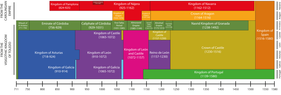
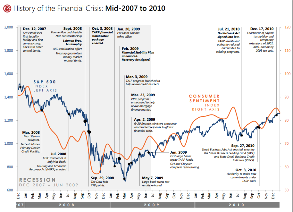
As a matter of fact, the presentation of changing magnitudes over time is the most frequent type of graphic visualization that we encounter in our daily lives. According to Edward Tufte, it is evident why this should be so: “With one dimension marching along to the regular rhythm of seconds, minutes, hours, days, weeks, months, years, centuries, or millennia, the natural ordering of the time scale gives this design a strength and efficiency of interpretation found in no other graphic arrangement.”2
However, as I intend to show in this article, there is absolutely nothing “natural” about the timeline and the graphic representations to which Tufte refers. Historically speaking, it is in fact quite a recent idea and took much persuasion and insistence to establish itself.
To ancient and medieval minds, today’s custom of beginning a diagram with a timeline would have appeared absurd – and in fact, I know of no ancient or medieval timeline, only of lines representing spatial extension and motion. The reason for this is that time was seen as a derivative notion. It measured change, while change took place in space, or at least between places. This is why Aristotle defined it as “the calculable measure or dimension of motion,” whereby the counting of this measure took place in the soul of a perceiving subject.3 Without motion, there was no time. And even if there was motion, without a perceiving and counting soul, there was still no time. According to Aristotle, the experience of continuous time depended on the continuity of motion, which in turn depended on topographic continuity.4
This is why Aristotle, and with him all of Antiquity and the Middle Ages, would be perplexed to see us draw a horizontal timeline as the x-axis above which we subsequently plot the changing values of speed, voltage, mortality or inflation. Put bluntly, in our practice, we plot change with respect to time, rather than deriving time from observed change, as everyone before the modern age did.
This does not mean, of course, that our ancient and medieval ancestors did not measure time. They clearly had calendars, counted days and decided to meet after dinner. But their calendars were based on celestial motions, that is, on the motions observed in the paths of sun, moon, and stars, which determined the divisions into months, days or hours. But celestial movements are nothing if not dislocations of celestial bodies from one place to another, with time once again being the derivative magnitude arising in the soul of the observer of these motions. Everyone agreed that when motions changed, time had to change, too. For medieval commentators, it was therefore evident that if the celestial bodies slowed down, time would also slow down, and if they stopped, so would time. That is why the idea of a flow of time that proceeded independently of motion would have seemed preposterous to them.
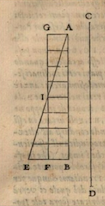
Historians of science have pointed for more than a hundred years to exceptional cases in which medieval diagrams supposedly did contain a temporal x-axis, and they celebrated these feats as ingenious anticipations of modern scientific diagrams. This is not the place to disprove all these claims.5 I will limit myself here to the most famous and applauded case, that of the so-called mean-speed theorem as supposedly illustrated by the 14th-century Nicolas Oresme. In the literature, we are usually shown the medieval diagram reproduced in figure 3 and then given a variant of figure 4 to explain its functioning.6
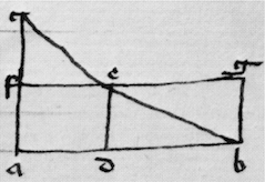
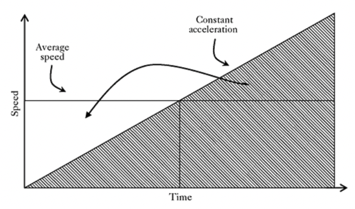
By flipping the 14th-century diagram so that it coincides with the ascending line of its modern reinterpretation, we obtain, according to our understanding, the following logic. A movement increasing regularly from velocity 0 to, say, a velocity of 10 km/h will have the same mean velocity as a movement that remains unchanged at the speed of the diagram’s middle point, that is, in our case, velocity 5km/h, as can be proven by simple geometry, the areas being equal. Since Pierre Duhem in 1912 first suggested it, everyone, including Philip Turetzky in his masterful study, Time, has interpreted the line a-d-b as a timeline: “The rate of change in a velocity […] can be represented geometrically by representing the extension of time by a base line […]. Time, then, is an enduring succession whose extension can be represented by a line.”7
But here, our own diagrammatic intuitions have inadvertently replaced Oresme’s! Not only is figure 3 taken from a chapter in Oresme’s Tractatus de configurationibus that has nothing to do with velocity, but is about corporeal qualities, but when he does turn to velocity, Oresme introduces a diagram that is not given in any of the extant manuscripts, explaining: “For example, let straight line AB be designed and let mobile D be moved through time EF in any way at all, whether it be in circular motion, rectilinear motion, or motion of alteration, and whether it be over line AB or over some other line.” His proof, carried out without the corresponding diagram, is opaque, nor is it evident where EF should be located. However, if the intended diagram bore any resemblance to figure 3 at all, as commentators have always assumed, then the line AB designated a distance, not time. Moreover, note that in our modern rendition of the diagram, where AB represents time, the moving body D has utterly disappeared from view: all we have is a geometrical correlation of speed with time. Oresme would have found the disappearance from our own diagrams of the moving body and the space it traverses bizarre.
This correction of our hitherto mistaken understanding of Oresme’s diagram actually explains two things that otherwise must remain paradoxical. The first is the 300-year absence of diagrammatic representations of time between Oresme and the early 17th century, which no one has been able to explain. The second is the astonishing difficulties that Galileo Galilei encountered when he did in fact need a timeline and, for the first time in the history of physics, drew one. His experiments had persuaded him that falling bodies accelerated according to time, not space, but when he first explained his law in 1604 to his friend Paolo Sarpi, he mistakenly drew a vertical line that represented the spatial fall, not the passage of time. As historians have observed, Thomas Harriot in England, Isaac Beeckman in the Netherlands and René Descartes in France and the Netherlands all made the same mistake. Why? Precisely because representing time as a line was counterintuitive to everyone then, just as it has become intuitive to us now. Later in his life, Galileo did devise diagrams to represent the law of acceleration, but he found this enterprise extremely difficult.
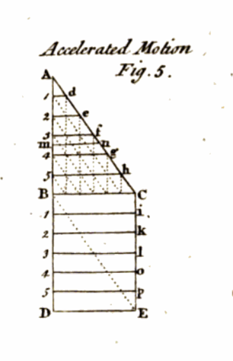
In figure 5, for example, we find him imitating Oresme’s diagrammatic style, representing the relation of regularly accelerated motion with constant motion by means of a triangle over a square, and measuring the increase in terms of areas.8 Since this is about falling bodies rather than a body moving through a landscape, Galileo turned Oresme’s figure 3 by 90o into the vertical direction of fall. But contrary to Oresme, Galileo now takes AB to represent time, whereby “each instant and all instants of time AB correspond to each point and all points of line AB.”9 But what is CD, then? It is the line of space, which Galileo places next to it, sheepishly watching the temporal line of the falling body next to it. It was inconceivable for Galileo to leave out of his diagram the actual body and the space that it traversed – a scruple that physics only lost in the second half of the 19th century. Evidently, he did not yet know how to combine time and space into a single graphic system, and the result is unsatisfactory, as AB and CD are functionally related.
But the history of science has been mistaken not only with respect to Galileo’s predecessors but also with respect to his successors. The literature assumes that the 17th century established our current diagrammatic order. This might have seemed logical, because when one adds to Galileo’s time-dependent law of fall Descartes’ coordinate system and Newton’s notion of absolute time, it should in fact be plausible to think that our modern diagrams were both visually ready for use and moreover philosophically legitimated. After all, for Newton, “[a]bsolute, true and mathematical time, of itself, and from its own nature flows equably without regard to anything external, and by another name is called duration.”10
But that is not how things went. A careful examination of thousands of woodcuts and copper plates in physics manuals from 1650 to 1850 forces me to conclude that physics teachers eschewed timelines throughout. The only exceptions to this avoidance are everywhere the laws of free fall and projectile motion, which functionally depend on time but which are routinely treated as if they constituted an embarrassment. More than 150 years after Galileo’s diagram and more than 100 years after Newton’s introduction of absolute time, physics manuals still did not treat time as a fundamental physical magnitude. Take Antonio Genovesi’s Elementa physicae experimentalis (1791):
Physics is the discipline that undertakes to contemplate the space of the entire universe in which we find ourselves, to the extent that this can be achieved, and all bodies that are contained in it; and therefore investigates the nature of bodies, their properties, differences, place, order, effects, and other phenomena, and their causes, modes, magnitudes, origins, ends, and finally their functions. The objects of physics are therefore spaces, bodies, movements.11
“Space, bodies, movements” – this is still the Aristotelian hierarchy of magnitudes, with time being viewed a subjective effect of motion in space. Or take William Nicholson’s Introduction to Natural Philosophy (London, 1790; Philadelphia, 1795). Its author pays no attention to time as a physical magnitude, but at some point discusses Galileo’s triangle constituted by a timeline AB and an increasing speedline of AC, with the increasing number of triangles designating the odd-number law of acceleration.12
Not only is this the only timeline in Nicholson’s textbook, but it still employs the old convention of matching time with areas denoting speed, rather than a coordinate system matching time to velocities. But many contemporary manuals did not even contain this single diagram. Friedrich Kries’ Lehrbuch der Physik (3rd ed. 1821) featured 41 woodcuts, but no representation of time.
If we want to understand why in the course of the 19th century conventions began to change, we have to take a fascinating detour that takes us out of the field of physics to history, historiography, and, even before that, chronology. A few decades before Galileo felt forced to draw a vertical, graduated timeline in analogy to the spatial line of fall, there was a group of humanist scholars who felt forced to invent an equally regular, graduated vertical time line, but for altogether different purposes.
The issue that chronologists wrestled with was that of mapping on to each other the different chronicles from ancient history – Egyptian, Greek, Persian, Jewish, Roman, etc. – so as to make them fit into a single, universal history. The main problem they encountered was that each culture had its own calendar, lunar, solar, or civil (i.e., dynastic or tax cycles). The earliest chronologists simply collated different chronicles next to each other, in numerical succession. But then, a map maker and cosmographer, Gerhard Mercator, first thought of a visually more convincing order, which, given his main, geographical preoccupations, cannot have been a coincidence. In his Chronologia, hoc est, temporum demonstratio exactissima ab initio mundi (1569), we find in fact the earliest representation (or “most exact demonstration,” as the title indicates) of time as a regular, onward moving line, graduated into regular intervals of 5 years. Mercator justified his innovation thus:
It was a deliberate choice that I continued the spaces of the years always in the same magnitude, even where there was nothing to inscribe. This equality is after all both appropriate and useful for who wants to calculate a certain number of years either forward or backward, without the pain of adding or subtracting. This increases the length and the price of this work, but this is compensated by its utility, and hence I opt for leaving this arrangement unchanged.13
Note that Mercator is not telling us that time itself has any regularity, but instead that the imposition of a visual and measurable regularity on the succession of events is useful – “even where there was nothing to inscribe.” Mercator, like everyone else, knew that, philosophically speaking, where nothing happens, there is no time to measure it.
Figure 7, crafted by one of Mercator’s successors, is truly baffling: it shows us time proceeding regularly and for several centuries before Creation has taken place. In order to fathom this philosophical impossibility, we must understand the following.14
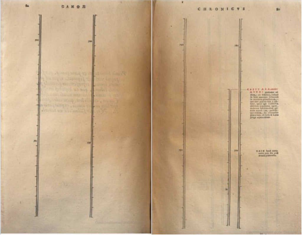
The Leiden humanist Joseph Justus Scaliger, who like all his colleagues wrestled with the various types of calendars, invented a method that he called the “Julian Period.” By this name he referred to an overarching cycle of 7980 years, the product of multiplying the 29 years of the solar cycle with the 19 years of the lunar cycle and the 15 years of the Roman cycle of indiction, which regulated taxation. The current cycle, in which we still live, began on January 1st, 4713 BCE. It was then that all three cycles were at point 0. However, given that Creation was taken to have occurred in 4004 BC, the beginning of the current Julian Period was a purely mathematical fiction, as no time could have existed before the world existed and heavenly bodies moved.
And yet, in his Opus chronologicum novum of 1619, the chronologist Ubbo Emmius began his timeline with that fictional 0-point. The result, shown in figure 7, is not only philosophically impossible, but also theologically subversive, but there it is: time starts running, with yearly marks, even in the absence of sun, moon or stars who could have defined these time units. Only hundreds of years later does real history begin, with the creation of the universe. As can be seen, that moment introduces a second timeline, to count the years since creation. Later, we will find additional ones, for the years since the foundation or Rome or the birth of Christ. Like Mercator before him, Emmius knew that he was not picturing time as a phenomenon. His “new form” of presenting history, which “placed the series and connections of times [of the various historical chronicles] before one’s eyes in a temporal order,” was above all “extremely useful to illustrate the matter, dispel the mist, establish certitude and place the series and connection of the times before one’s eyes.”15 Once more, the timeline was offered as a solution to a practical problem. It was usefulness, not truthfulness, that mattered.
As in the case of Galileo’s diagrammatically depicted law of fall, one might have expected that the chronologists’ handy convention established today’s ubiquitous graphic conventions. But once more, this inference would be mistaken. More than 200 years passed before the same idea, but now in horizontal form, was reproposed. In the second half of the 18th century, various proposals were put forward to display information graphically, along a timeline. This happened first in historiography, with past events mapped in synopses along a timeline, and subsequently in economics, with data correlated as data points in coordinate systems, the timeline now finally functioning as the x-axis. And, once again, it is conspicuous that their manufacturers felt that they had to justify their graphic tools to their readers (or beholders), not only because they felt that their graphic typologies were novel, but because they also realised that a spatial representation of time was not philosophically legitimate.
In the domain of historiography, the main innovator was Joseph Priestley, who in 1765 presented an enormous Chart of Biography, of which figure 8 is a mere ‘specimen’.16
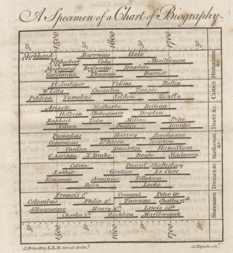
In their study of the representation of history in charts, Rosenberg and Grafton describe this chart as nothing less than a “watershed,” as “it was the first chart to present a complete and fully theorized visual vocabulary for a time map, and the first to successfully compete with the matrix as a normative structure for representing regular chronology.”17
To us, the logic of this representation is obvious, but Priestley felt that he had to justify it in a thousand ways. He conceded that “time” was merely “an abstract idea” that could not be represented visually. But, he insisted, it shared a sufficient number of qualities with space to allow, by analogy, for a representation in terms of graduated lines. And so, even though time was “not the object of any of our senses, and no image can properly be made of it,” nevertheless, “because it has a relationship to quantity […], it admits of a natural and easy representation in our minds by the idea of a measurable space, and particularly that of a line.”18
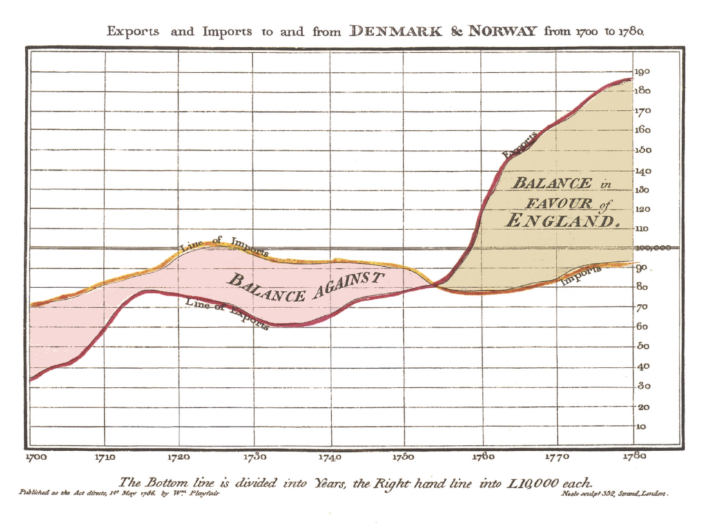
That by drawing a line, one subjected time to a spatial understanding was also obvious to William Playfair, maybe history’s most fruitful innovator of diagrammatic modes of representation. When in 1786, he introduced statistical “charts” in his Commercial and Political Atlas, it was not just the title word “Atlas” that referred to spatial mapping, but his representation of data in coordinate systems explicitly rested on geographical tools, as they had, centuries before, for Mercator.
In figure 9, we have, for the first time, a coordinate system with a timeline as the x-axis and some values mapped along the y-axis.19 Playfair was aware that “[t]o those who have studied geography, or any branch of mathematics, these charts will be perfectly intelligible. To such, however, as have not, a short explanation may be necessary.”20 As for “geography,” that is indeed where the idea of “mapping data” comes from; as for “any branch of mathematics,” it refers to geometry or to the diagrammatic representation of functions. What was new, however, was the substitution of the spatial dimension by a temporal one. Like Priestley, who wished to capture the “flux” of history along a timeline, Playfair also insisted that his mode of representation might not be philosophically defensible, but was eminently useful.
The amount of mercantile transactions in money, and of profit or loss, are capable of being as easily represented in drawing, as any part of space, or as the face of a country; though, till now, it has not been attempted. Upon that principle these Charts were constructed; and, while they give a simple and a distinct idea, they are as near accuracy as is in any way useful.21
This time around, the innovation stuck. By the end of the 18th century, both the historical chart and statistical mapping had become common, and with it the notion that one could accept time as a regular, progressive baseline. Oresme’s line a-d-b of a vehicle’s progression had now truly turned into a line depicting the flux of time.
Immanuel Kant documents nicely how the establishment of this new visual convention began to influence philosophy. Kant, pace certain hasty summaries of his doctrine, did not treat time and space analogously. For him, time was the intuition of inner sense, which stands in a relation of subordination to space, the intuition of the outer sense. Kant remained essentially Aristotelian when describing motion as taking place in space, with the conscious subject observing that motion and in the process experiencing time. In a key passage of his Critique of Pure Reason, he states that the best way in which we can present change as experienced internally is by drawing a straight line. The argument runs as follows:
For space alone is determined as permanent, while time, and therefore everything that is in inner sense, is in constant flux. Secondly, in order to exhibit alteration as the intuition corresponding to the concept of causality, we must take as our example motion, that is, alteration in space. […] The intuition required [for capturing change] is the intuition of the movement of a point in space. […] For in order that we may afterwards make inner alterations likewise thinkable, we must represent time (the form of inner sense) figuratively as a line, and the inner alteration through the drawing of this line (motion), and so in this manner by means of outer intuition make comprehensible the successive existence of ourselves in different states.22
This is not the place to unpack this quote fully, but it should be obvious that it documents Kant’s awareness that the drawing of a line is a mere tool to build our intuition of time, as well as his conviction, which no author of previous centuries would have shared, that it was an obvious and in fact even “required” intuition. Henri Bergson, a century later, would loudly lament this erroneous mixing up of spatial and temporal intuitions, believing them to be due to the projection of memories of different spatial situations onto a single space, whose multiplicity is then understood – mistakenly – as the flux of time. “Space used to this effect is exactly what one calls homogeneous time.”23
As we have heard above, physics resisted the introduction of the timeline well into the 19th century. The earliest explicit description that I have found occurs in Ernst Mach’s Compendium der Physik für Mediziner (1863). Intended for medical students, this physics textbook starts pedagogically by explaining how physicists reason: they first define the variables they want to examine, then collect data that they hope will yield underlying patterns, which they then express in functions of the type y = a + bx + cx2 + dx3 + … . According to Mach, it is helpful for scientist to render the functions, once found, visual (anschaulich machen), by translating them into coordinate systems. To document these steps, Mach takes the case of motion. Proceeding with didactic patience, he starts with the simple case of regular motion, that is, with the case in which in each second of time (t), a given body traverses the same interval (c) of space (s), so that s = ct. Having given the relation in an algebraic expression, Mach switches to the register of geometry:
In order to represent the law of regular motion graphically also, we inscribe (as in Figure [10]) the times as vertical lines [Abszisse] along OT, and the intervals as horizontal lines [Ordinaten] along OS, and in this manner, we obtain, by connecting all the endpoints of the horizontal lines, a straight line.24
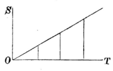
This is old Oresme’s diagram, but with the crucial difference that we finally do have a time axis, next to a spatial axis, rather than a relation of the object’s path to the intensities of speed. But, as Oresme would have pointed out, the moving object itself has entirely disappeared from the diagram.
The last twist of this story, and the one with which we bid adieu to the reader, is this. Only 40 years after Mach and his colleagues had started to treat time as a horizontal x-axis above which physical data could be plotted, Albert Einstein explained to the astonished world that time was not an independent dimension at all. Since then, theoretical physicists working on time offer us, so as to help our imagination, Minkowski space-time diagrams or past and future light cones intersecting in spatial planes. But if one had expected relativity theory to shoo the timeline out of existence, one would once more have been mistaken. In fact, we find it everywhere, thriving.
What does this story tell us? It tells us a number of things. To begin with, our natural habit of depicting, and imagining, time as a regular horizontal line is a pure convention, and a recent one at that. It is moreover philosophically ungrounded, as everyone until 1800 knew and some, like Bergson, pointed out even later. It is also physically misleading, as everyone before Newton and everyone after Einstein recognized. And yet, it is apparently so helpful in organizing information for us that we won’t let go of it. For those who are aware of this situation, this is a typical case of what Hans Vaihinger has analyzed in terms of the scientific utility of concepts “as if” (Die Philosophie des Als Ob, 1911). For everyone else, this historically recent convention has become an intuition of such a force that its naturalness seems obvious.
Christoph Lüthy is professor in the History of Philosophy and Science at Radboud University, Nijmegen (The Netherlands). He works on the transformation of natural philosophy into modern science, as well as on the logic of scientific imagery and the history of atomism.
- Figure 1: https://commons.wikimedia.org/wiki/File:Timeline_of_Kingdoms_of_the_Iberian_Peninsula_(711-1580)_(ENG).svg. Figure 2: U.S. Department of Treasury, “The Financial Crisis Five Years Later: Response, Reform, and Progress” (September 2013). ↩︎
- Edward R. Tufte, The Visual Display of Quantitative Information, 2nd ed. (Cheshire, CT, 2001), 28. ↩︎
- Aristotle, Physics, transl. Ph. H. Wicksteed and F. M. Cornford (Loeb Classical Library, 228 and 255) (Cambridge, MA, 1929, 1930), IV, 219b2–3. ↩︎
- Ibid. IV, 219a11–13. ↩︎
- For a full treatment, see my “The Late Origins of the Timeline, or: Three Paradoxes Explained,” Annals of Science, 82 (2025), 1–43. ↩︎
- Figure 3: Oresme, Tractatus de configurationibus qualitatum et motuum (1350s). British Library, Sloane 2156, fol. 164r. Figure 4: “Nicole Oresme’s proof of the mean speed theorem in graphical form,” in James Hannam, God’s Philosophers. How the Medieval World Laid the Foundations of Modern Science (London, 2009), fig. 14. ↩︎
- Turetzky, Time (London, 1998), 67–68. ↩︎
- Figure 5: Galileo Galilei, Discorsi e dimostrazioni matematiche intorno a due nuove scienze (Leiden, 1638), 10. ↩︎
- Galileo Galilei, Two New Sciences, transl. Stillman Drake, 2nd ed. (Toronto, 1989), 165. ↩︎
- Isaac Newton, scholium to the definitions in Philosophiae Naturalis Principia Mathematica, Bk. 1 (London, 1689); transl. Andrew Motte (London, 1729), rev. Florian Cajori (Berkeley, 1934). ↩︎
- Antonio Genovesi, Elementa physicae experimentalis (Naples, 1791), 1. Translation mine. ↩︎
- William Nicholson, An Introduction to Natural Philosophy, 2nd ed. (Philadelphia, 1795), 30–32. Figure 6: Ibid., plate 1, fig. 5. ↩︎
- Gerhard Mercator, Chronologia (Cologne, 1569), 4v. Translation mine. ↩︎
- Figure 7: Ubbo Emmius, “Canon chronicus plenior,” 320, in Emmius, Opus chronologicum novum, pluribus partibus constans; elaboratum & concinnatum (Groningen, 1619). ↩︎
- Emmius, Opus chronologicum novum, *2v–*3v. ↩︎
- Figure 8: Priestley, “A Specimen of a Chart of Biography,” in Priestley, The History and Present State of Electricity with Original Experiments (London, 1767). ↩︎
- Daniel Rosenberg and Anthony Grafton, Cartographies of Time. A History of the Timeline (Princeton, NJ, 2012), 19. ↩︎
- Joseph Priestley, “Description of a Chart of Biography,” in Priestley, The Theological and Miscellaneous Works, ed. Towill Rutt (New York, 1972), vol. 24, 465. ↩︎
- Figure 9: William Playfair, The Commercial and Political Atlas, Representing, by Means of Stained Copper-Plate Charts, the Progress of the Commerce, Revenues, Expenditure, and Debts of England, 3rd ed. (London, 1801). ↩︎
- Ibid., ix. ↩︎
- Ibid., xiv. ↩︎
- Immanuel Kant, Critique of Pure Reason, transl. Norman Kemp Smith (London, 1929), B 291–92. ↩︎
- Henri Bergson, Essai sur les données immédiates de la conscience (Paris, 1889), 66. Translation mine. ↩︎
- Ernst Mach, Compendium der Physik für Mediziner (Vienna, 1863), 20. Figure 10: Ibid., 21. ↩︎